Sound Waves and Subsurface Vision
Controlled seismic sources generate elastic waves that propagate through rock strata. These waves partially reflect at boundaries where acoustic impedance changes abruptly.
The reflected wavefield carries information about depth, geometry, and elastic properties of rock layers. Recording this field densely along survey lines is the first step toward subsurface imaging.
Modern acquisition uses thousands of receivers to capture the full wavefield in three dimensions. Each shot generates a seismic trace; assembling millions of traces creates a massive dataset. The challenge lies in extracting coherent signal from noise and converting travel times into accurate depth positions. Seismic waves obey the same physical laws as light, but their velocities are orders of magnitude lower, making timing precision critical. The reflection coefficient at an interface depends on the contrast in density and wave speed, a relationship that forms the quantitative basis of amplitude interpretation.
From Echoes to Images
Raw field records are merely voltage‑versus‑time series contaminated by multiples, ground roll, and random noise. Deconvolution compresses the source wavelet and attenuates short‑period multiples, improving temporal resolution.
After deconvolution, each trace is sorted into common‑midpoint gathers. Coherent signal enhancement through stacking requires accurate velocity analysis. Incorrect velocities misalign reflections and degrade the final image.
Normal moveout correction removes the offset‑dependent travel‑time delay, flattening reflections across a gather. The hyperbolic travel‑time curve is fitted during velocity picking, a step that still demands skilled human interpretation despite automated algorithms.
Stacking sums the corrected traces, boosting primary reflections while reducing uncorrelated noise and multiples. A single stacked trace represents the zero‑offset response of the earth. Modern processing flows also include surface‑consistent amplitude corrections and spectral balancing. Stacking alone, however, produces a blurred image; spatial positioning errors remain because the recorded wavefronts are assumed to come from vertically travelling paths. This assumption is valid only for flat, horizontal layers.
The following sequence represents the fundamental processing workflow applied to nearly every marine or land seismic survey before migration:
- Geometry assignment and trace editing Step 1
- Deconvolution (spike or predictive) Step 2
- Velocity analysis and NMO correction Step 3
- Residual statics correction Step 4
- CMP stacking Step 5
These steps transform raw shot records into a stacked section that approximates a normal‑incidence reflectivity profile. The stacked section still suffers from misplaced dipping events and diffractions, which require the focusing operation known as migration to be properly positioned.
Migration: Focusing the Blur
Migration fundamentally repositions recorded reflection events to their true subsurface coordinates. The process corrects for dip‑dependent misalignment and collapses diffractive energy into discrete points.
Stacked sections assume reflections originated vertically, an approximation that blurs dipping layers and faults. Migration solves this by using a velocity field to back‑propagate the recorded wavefield, achieving accurate spatial positioning of geological boundaries. A clear example is the collapse of a diffraction hyperbola into a single apex.
Kirchhoff migration, a ray‑based method, integrates amplitudes along calculated travel‑time curves; it remains popular for prestack time imaging. Wave‑equation algorithms such as one‑way phase shift plus interpolation handle moderate lateral velocity variations. For complex geologies—especially subsalt provinces—reverse time migration solves the complete two‑way wave equation and correctly images turning waves and multiples. All these approaches share a critical dependence on the velocity model; inaccuracies directly misposition reflectors and defocus fault planes. Contemporary workflows thus tightly couple migration with full‑waveform inversion or reflection tomography to iteratively refine the velocity field and the migrated image.
Beyond 2D: Volumes and Voxels
Three‑dimensional seismic acquisition records the wavefield over a dense areal grid, producing a data cube whose axes are inline, crossline, and two‑way travel time or depth. Each elemental unit in this cube is a voxel that carries an amplitude value, transforming seismic interpretation from profile‑wise inspection to true volumetric analysis.
Interpreters can now slice the volume horizontally, creating horizon slices or proportional slices that display paleo‑depositional surfaces. Chronostratigraphic slicing allows direct visualisation of channel systems and submarine fans without manual picking of every reflector. Seismic geomorphology emerged from this capacity to see ancient landscapes in three dimensions.
Before extracting quantitative attributes, one must understand the fundamental sampling parameters of a seismic volume. Inline and crossline spacing defines the lateral resolution; typical bin sizes range from 6.25 m in high‑resolution surveys to 25 m in conventional exploration. Vertical sample intervals are commonly 2 or 4 ms. The table below lists four widely used volumetric attributes, each derived from different physical properties of the reflected wavefield.
| Seismic Attribute | Primary Application | Physical Basis |
|---|---|---|
| Acoustic impedance | Lithology prediction, porosity estimation | Product of density and P‑wave velocity |
| Instantaneous frequency | Gas accumulation, thin‑bed tuning | Time derivative of instantaneous phase |
| Coherence | Fault and fracture mapping | Cross‑correlation similarity between traces |
| Curvature | Stress‑related fracture prediction | Second derivative of reflector surface |
Voxel‑based representation unlocks geostatistical and machine‑learning workflows that were impractical with 2D profiles. Seismic inversion transforms amplitude voxels into elastic property volumes—acoustic impedance, shear impedance, density—that relate directly to rock physics. Simultaneously, convolutional neural networks ingest small 3D sub‑volumes to segment salt bodies, classify facies, or predict well‑log properties. These algorithms exploit the full spatial context around each voxel, learning patterns invisible to conventional single‑trace analysis. The enormous size of modern surveys, however, requires specialised data structures and parallel computation to handle petabyte‑scale volumes efficiently.
Why Seismic Resolution Matters
Resolution in seismic imaging is quantified by the minimum separation at which two reflectors can be distinguished. It governs whether thin reservoirs and small faults are detected or remain invisible.
Vertical resolution depends on the dominant wavelength and is often approximated by the Rayleigh criterion (λ/4). Thin beds below the tuning thickness produce composite reflections whose amplitude varies linearly with thickness—a relation exploited for net‑pay estimation. The Widess limit (λ/8) defines the theoretical lower bound where tuning gives way to constant waveform.
Lateral resolution is controlled by the Fresnel zone diameter before migration and by the migration aperture afterward. Post‑migration resolution approaches half the dominant wavelength in ideal conditions, but practical issues—velocity uncertainty, irregular illumination, and acquisition footprint—often degrade it. Consequently, features such as pinch‑outs, channels narrower than the bin size, and sub‑seismic faults remain unresolved. Accurate resolution assessment directly impacts reserve estmation and drilling risk; overconfident interpretation of under‑resolved data has led to numerous dry holes. Vertical resolution and lateral resolution together determine the geological detail recoverable from a seismic volume.
Full‑Waveform Inversion
Full‑waveform inversion iteratively minimizes the difference between observed and synthetic seismograms, extracting high‑resolution quantitative models of subsurface parameters. It exploits the entire wavefield—reflections, refractions, multiples, and diving waves—not merely traveltimes.
- 1. Initial model — background velocity from tomography or migration velocity analysis
- 2. Forward modelling — solving the wave equation (acoustic, elastic, or viscoelastic)
- 3. Residual calculation — sample-wise difference between recorded and modelled wavefields
- 4. Adjoint gradient — back-propagation of residuals through the time-reversed wavefield
- 5. Model update — steepest descent, Gauss-Newton, or L-BFGS optimisation
- 6. Iteration — until convergence or data misfit reduction stalls
The method places extreme demands on low‑frequency content, long offsets, and accurate physics. Without frequencies below 3 Hz, the inversion often converges to a local minimum.
Recent advances incorporate elastic and visco‑acoustic wave equations, enabling simultaneous recovery of P‑wave velocity, S‑wave velocity, density, and attenuation. Time‑lagged FWI and reflection FWI mitigate the cycle‑skipping problem by refocusing on specific wave types. Although computationally expensive—typically requiring hundreds of wave‑equation solves—GPU acceleration and clever source‑encoding strategies have made 3D FWI feasible for industrial surveys. The resulting velocity models resolve salt flanks, gas clouds, and thin layers with unprecedented fidelity, directly improving subsequent depth imaging and pore‑pressure prediction.
Machine Learning in Seismic Processing
Machine learning algorithms learn complex, non‑linear mappings directly from seismic data. Convolutional neural networks and gradient‑boosted trees now automate fault detection, facies classification, and even first‑break picking.
Supervised techniques require extensive labelled examples, often derived from well logs or manual interpretation. Transfer learning and semi‑supervised approaches reduce this dependency by leveraging synthetic data or unlabelled volumes. The following table summarises prominent ML applications and their characteristic input features.
| Application | Learning Paradigm | Primary Input Features | Typical Output |
|---|---|---|---|
| Fault detection | Supervised (CNN) | Seismic amplitude patches, coherence | Fault probability volume |
| Facies classification | Supervised / semi‑supervised | Post‑stack amplitudes, attribute blends | Lithofacies map |
| First‑break picking | Supervised (LSTM, CNN) | Raw shot gathers, offset information | First‑arrival times |
| Velocity model building | Physics‑informed / GAN | Shot gathers, migration images | High‑resolution velocity field |
| Noise attenuation | Self‑supervised (autoencoders) | Noisy common‑shot gathers | Denoised seismic traces |
Despite remarkable progress, several obstacles impede routine industrial adoption. Networks trained on one basin frequently fail when applied to another without extensive fine‑tuning—a symptom of the domain shift problem. Explainable artificial intelligence methods are therefore gaining prominence, as they allow interpreters to verify that models learn geologically plausible features rather than noise or acquisition ffootprints. Simultaneously, the integration of physical constraints into deep learning architectures is accelerating.
Physics‑informed neural networks embed the wave equation directly into the loss function, enabling inversion with minimal labelled data while honouring fundamental propagation principles. Hybrid workflows that combine full‑waveform inversion with generative adversarial networks now produce high‑resolution velocity models from incomplete surveys. Such synergies between data‑driven and physics‑driven paradigms represent the most promising direction for computational geophysics in the coming decade.